The Virtual Geoscience Revolution: From William Smith to Lidar
Contents
The Virtual Geoscience Revolution: From William Smith to Lidar
In 1799 a surveyor called William Smith published the World’s first geological map and fundamentally changed the way in which geologists envisaged the subsurface [WV01]. For the next 200 years, field geologists did as Smith had done, tracing geological boundaries on the ground and used ink pens and coloured pencils to record the surface expression of the geology onto paper and maps (Figure 3A). Even today, the largest single component of any undergraduate degree in the UK is the “mapping project”, where students make detailed maps of a selected area. There can be very few sciences where there have been no significant changes in the basic data collection methods for over 200 years. However, since the turn of the 21st Century we have seen a quiet revolution in the way in which field data are collected, analysed, and displayed. We call this the Virtual Geoscience Revolution and it has come about in a number of discrete phases, each of which have resulted from the development of a number of distinct but parallel technologies.
Stage 1 – Satellites and GPS.
It’s not easy to remember a world without GPS, but in the mid 1990’s to locate yourself on a map, orienteering with a compass and landmarks was standard practice. Early GPS units were cumbersome and inaccurate, but towards the end of the 90’s small handheld units became affordable and usable in the field. The application still relied on transposing coordinates onto a paper map and had errors that meant they were not good enough for detailed mapping, but this was the first stage of digital data collection. At the same time, more expensive differential GPS systems started to appear that relied on stationary base stations to correct satellite drift (post-processed or in real time) from a rover unit position. For the first time it was possible for a geologist to trace a field boundary and record it digitally.
Stage 2 – Early Virtual Outcrops
Whilst walking out geological boundaries was the start of digital mapping, it was time consuming. Shortly afterwards, a whole new school of digital geology was born. With a virtual outcrop, the entire outcrop is captured in a 3D picture where the exact location of every pixel is recorded. The earliest attempts (that we are aware of) came when researchers at Statoil tried to use photogrammetry (more about that later) to capture cliffs in Utah and Spain as part of the original SAFARI Project [DFaltHoy+93]. These attempts failed because, while the concept was good, computer hardware and storage space had yet to catch up.
The first practical virtual outcrops came in the early 2000’s with the work of Carlos Aiken and others at UT Dallas [XAB+00]. A robotic Total Station was used to record the location of a few tens of points on a cliff face. This provided a framework onto which photogrammetry was used to produce a photorealistic model of the outcrop. Whilst this work was pioneering, it did not receive the attention that it deserved at the time.
Stage 3 – LIDAR
Soon after Aiken et al. were building their models, terrestrial lidar appeared on the scene. Designed for architectural scanning, the first application in Geology was by Jerry Bellian and Dave Jeanette at the Bureau of Economic Geology [BKJ05]. A lidar system records the time of flight of a rapidly pulsed laser beam shot at cliff faces (several tens of thousands points per second – up to a million today) and calculates a spot position. This produces a point cloud of millions of georeferenced points that accurately recorded the shape of the outcrop. The subsequent addition of a digital camera meant the point cloud could be coloured to produce a highly accurate but lowish resolution 3D image. The 3D image is significantly improved when the point cloud is triangulated and meshed to create a solid surface onto which the photographs could be draped. The virtual outcrop, as we know it today was born (Figure 3B).
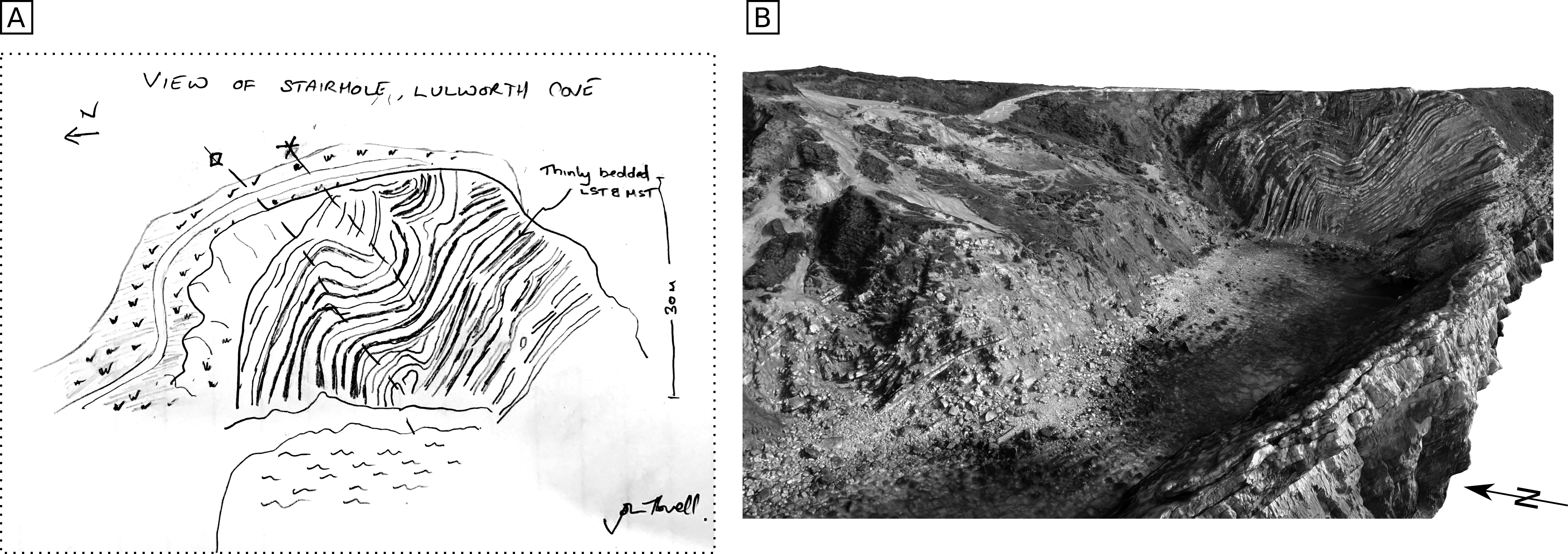
Fig. 3 Lulworth Cove, UK. A. Typical sketch with annotations that a geologist would create rom field observations B. 3D view of a virtual outcrop of the same outcrop in the field sketch.
References
- BKJ05
J.A. Bellian, C. Kerans, and D.C. Jennette. Digital Outcrop Models: applications of Terrestrial Scanning Lidar Technology in Stratigraphic Modeling. Journal of Sedimentary Research, 75(2):166–176, mar 1 2005. URL: http://dx.doi.org/10.2110/jsr.2005.013, doi:10.2110/jsr.2005.013.
- DFaltHoy+93
T. Dreyer, L.-M. Fält, T. Høy, R. Knarud, R. Steel\textsection , and J.-L. Cuevas. Sedimentary Architecture of Field Analogues for Reservoir Information (SAFARI): A Case Study of the Fluvial Escanilla Formation, Spanish Pyrenees, pages 57–80. Blackwell Publishing Ltd., 4 1993, [Online; accessed 2021-07-26]. URL: https://onlinelibrary.wiley.com/doi/10.1002/9781444303957.ch3, doi:10.1002/9781444303957.ch3.
- WV01
Simon Winchester and Soun Vannithone. The map that changed the world: William Smith and the birth of modern geology. HarperCollins, 1st ed edition, 2001.
- XAB+00
Xueming Xu, Carlos L. V. Aiken, Janok P. Bhattacharya, Rucsandra M. Corbeanu, Kent C. Nielsen, George A. McMechan, and Mohamed G. Abdelsalam. Creating virtual 3-D outcrop. The Leading Edge, 19(2):197–202, 2 2000. URL: http://dx.doi.org/10.1190/1.1438576, doi:10.1190/1.1438576.