Prototype colourmaps for fault interpretation
Prototype colourmaps for fault interpretation
This article describes ongoing work to build an interactive web app for colourmaps to highlight subtle seismic features such as faults. Standard grayscale is already quite effective at highlighting low-amplitude events to aid in the recognition of subtle terminations [1]. However, grayscale can be improved for this purpose by dynamically varying the Lightness contrast to be high in the central portion of the colourmap and low at the ends.
This can be accomplished in Hue-Saturation-Lightness colour space using a logistic sigmoid curve [2] for Lightness. Hue and Saturation are then set to zero and the colourmap is converted from HSL to RGB.
There are two stages in the app creation process: developing the individual elements separately (the sigmoid function, plotting routines, et cetera), and assembling them into a user interface. The code below shows the function that creates the sigmoid Lightness curve and how it is called.
def sigmoid_demo(x,c,w):
    sgm = 1/(1+np.exp(-(x-c)/w))
    return (sgm-min(sgm))/(max(sgm)-min(sgm))
x = np.linspace(0,10,256)
l_sigm = sigmoid_demo(x,5,1)
h_sigm = np.zeros(256)
s_sigm = np.zeros(256)
The shape of the sigmoid is controlled by the equation in line 02 using two parameters: c, the position of the central ramp, and w, its width (which in turn determines the contrast). x is the sample number, defined in line 04 prior to calling the function. The resulting curve is normalized in line 03 to the range 0-1 (Lightness range for Matplotlib colourmaps). The function is called in line 05 to create a 256x1 Lightness array. The commands in lines 06 and 07 create two 256x1 arrays of zeros for Hue and Saturation.
The Jupyter notebook Sigmoid_function_experiments.ipynb demonstrates the effects of varying the parameters c and w in different ways.
The full app prototype, built using the interactive tools from the IpyWidgets module, is available in the Jupyter notebook Sigmoid_app_static_new.ipynb. A screen capture is shown in Figure 1. (Note that in this notebook, the parameter c is held fixed at a value of 5.)
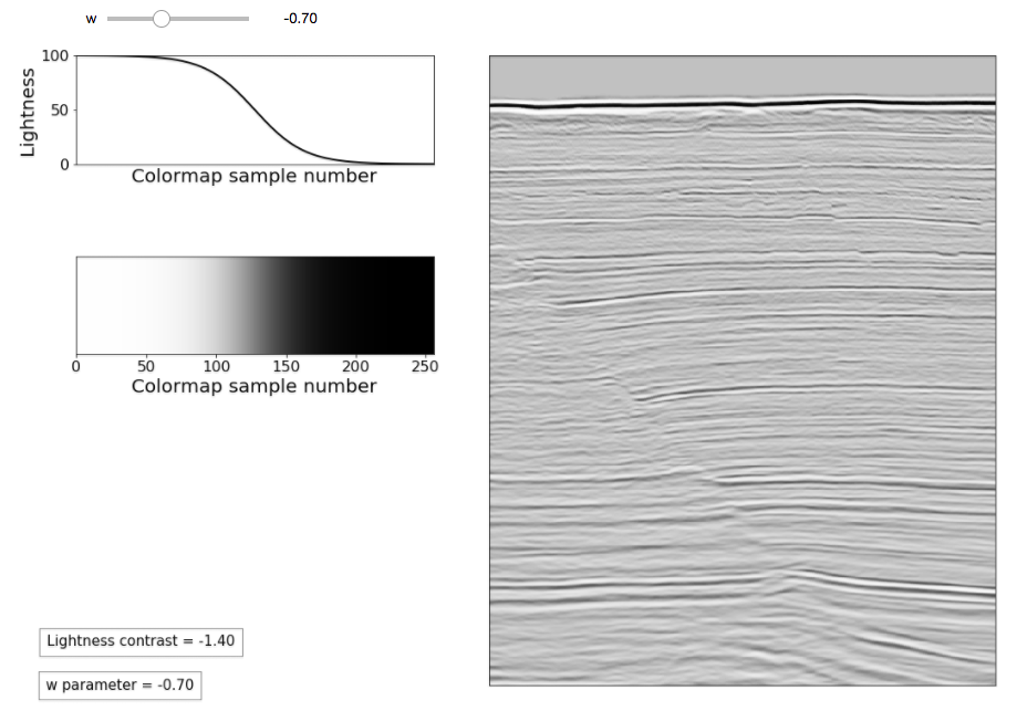
Figure 1 – Sigmoid grayscale app prototype.
In Figure 1, the sigmoid Lightness curve is plotted in the top-left panel. The resulting colourmap, created using tools described in [3], is plotted in the middle-left panel. The right panel is a demo seismic section with faults – crossline 1155 from the Penobscot F3 3D, the same as used in [4]. The sample-to-sample Lightness contrast in the central portion of the colourmap is calculated as:
(l_sigm \[128\]- l_sigm\[127\])\*100
In the example in Figure 1, the contrast is -1.40 (negative) since Lightness decreases with increasing sample number. As a reference, the contrast in standard grayscale is about 0.4. To make the interface work, all elements are grouped together in a single function called sigmoid_demo in Sigmoid_app_static_new.ipynb. The last element in the prototype, in the top-left in the figure, is an interactive slider created by this line at the end of the notebook:
rslt = interactive(sigmoid_demo, w=FloatSlider(min=-2.7, max=2.7, step=0.1, value = 1))
The command calls the sigmoid_demo function, specifying a range for parameter w, for the purposes of this demo chosen to be from -2.7 to 2.7 in steps of 0.1. The parameter c is held constant since we want an antisymmetric colourmap. sigmoid_demo pre-generates all the results at once and activates the slider, allowing users to interact with the tool. Using interactive also allows access to the returned colormap array in later cells so that it can be exported.
As an aside, an alternative to creating a sigmoid colourmap would be to directly modify the seismic amplitudes by applying a sigmoid stretch. Although I prefer the colourmap approach, I show how to do this in a third notebook named Scaling_seismic_sigmoid.ipynb.
I plan to build a future, final version of this app using Panel (https://panel.holoviz.org/). This will include the ability to save the colourmap in a variety of formats and to import a user-defined seismic section in either SEGY or ASCII format.
References
[1] Brown, A. (2012). Interpretation of Three-Dimensional Seismic Data. SEG Investigations in Geophysics, no. 9, 7th edition.
[2] Sigmoid Function, Wolfram Mathworld. http://mathworld.wolfram.com/SigmoidFunction.html
[3] Niccoli, M. (2014) Evaluate and compare colormaps. The Leading Edge 33, no. 8, 910–912. Open access at: https://github.com/seg/tutorials-2014#august-2014
[4] Bianco, E. (2014) Well tie calculus. The Leading Edge 33, no. 6, 674-677. Open access at: https://github.com/seg/tutorials-2014#june-2014